Microsoft Excel (Spreadsheet 10th Class)
Q:- What is Auto sum? How to use to Auto sum in Cells?
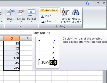
Ans:- Auto sum is used for adding the values given in cells automatically without writing the formula to perform the operation.
Sum is one of the functions available in the spreadsheet to perform the addition of selected numbers in the sheet.
Autosum automatically select values around the cells either horizontally or vertically.
- Create a New or Existing Worksheet.
- Enter the desire numeric number in cells
- Then select the all cells which want to add.
4. Click the option Auto sum under the Editing group in the Home tab.
Q:- What is Conditional Formatting?
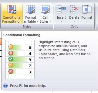
Ans:- Condition Formatting(CF) is a tool that allows you to apply formats to a cell or range of cells. Conditional formatting changes depending on the value of the cell or the value of a formula.
Condition formatting allows us to change the formatting (font color, border size, shadow) of the cells based on values in it.
In Excel, Conditional formatting enables us to highlight cells with a certain color.
Conditional formatting available under style group in Home Tab.
Q:- Explain the Freeze a row or column in Excel?
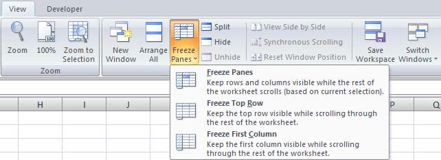
Ans:- Freezing rows and columns is a feature in a spreadsheet. When we want the header to remain constant while scrolling through the data, we can do the features of freezing in a spreadsheet.
To freeze the rows or columns do the following –
- Open a new or existing spreadsheet.
- To freeze rows or columns click on Freeze panes option available under window group in the View tab.
Spreadsheet 10th Class
Q:- Explain the Page Layout. How to set the layout of a page in Excel?
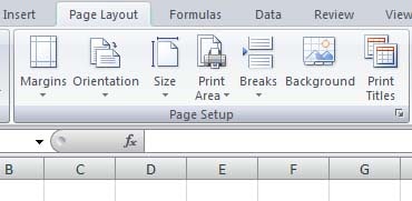
Ans:- Spreadsheet software provides various page layout options for organizing pages using the page layout option. Page layout is the term used to describe how each page of our document will appear when it is printed.
Page layout option
| · Margins | · Orientation Page Headers and Footers | · Hide or Display grid lines |
| · Size of the page | · Define the print area | · Specify the background |
Q:- Define a Workbook, Worksheet.
Ans:-A workbook is the MS Excel file in which you enter and store related data.
A worksheet is collection of cells on a single sheet. It is also known as Spreadsheet. we can manipulate the data in easy way in the worksheet. Each workbook can contain many worksheets.
Q:- How many types of views in the spreadsheet?
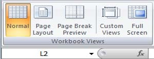
Ans:-There are five types of views available in the spreadsheet.
- Normal:– This is the default view of spreadsheet application. It’s a collection of cells arranged in the work area.
- Page layout:– use page layout view to see where pages begin and end, and to add headers and footers.
- Page break preview:- This option is similar to the Page Layout option except we can set the area that is to be set as a page after inserting a page break.
- Custom view:– If we would like to view selected areas of a document. We can use the custom view option.
- Full-screen view:– If the select full-screen view then the workbook covers the entire screen. All tabs are hidden from view.
Spreadsheet 10th Class
Q:- Write the short note of Range and Range name.
Ans:- Range:- A Range is a group of blocks of cells in a worksheet that has been selected or highlighted.
When cells have been selected by black border or outline. Normally only one cell in worksheet with black outline.
Range names – A named range is just a human-readable name for a range of cells in Excel. For example, if we name the range A1: A50 data. we can use MAX to get maximum value with simple formula.
Q:- What is Chart?
Ans:- A chart is a powerful tool that allows you to visually display data in a variety of different chart formats. A Spreadsheet enables us to create, modify and format charts based on the data given in the spreadsheet.
We can represent data or functions in tabular form with the help of Chart. A Chart is graphical representation of data, in which data is represented by some types of chart i.e bar chart, line chart and column chart.
Q:- List of Seven Chart Elements.
Ans:- Chart has many elements, only some of the elements are displayed by default.
| 1. Chart Area of the chart | 2. Plot Area of the chart | 3. Data points |
| 4. Horizontal and vertical axis | 5. Legend | 6. Chart and Axis Title |
| 7. Data Label |
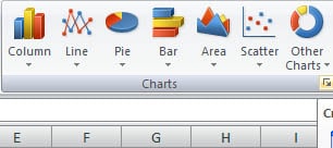
Q:- List Six chart types available in the spreadsheet.
Ans:- Excel chart helps is to display data visually in the most meaningful way.
- Bar Charts
- Column Chart
- Line Chart
- Pie Chart
- Area Chart
- Scatter Chart
Spreadsheet 10th Class
Q:- What is Sorting and Filtering? How to sort and filter data in Excel?
Ans:- Sorting:- Sort is a feature that helps arrange the selected data either in an ascending or descending order. We can quickly reorganize a worksheet by sorting your data. For example, we could organize a list of contact information by last name. Data can be sorted alphabetically, numerically and in many other ways.
Filter:- Filter is a feature used for extracting particular data using some conditions. If we want to certain data displayed, we can use Filtering tool in spreadsheet.
The basic filter allow to view specific rows in Excel while hiding other rows.
Q:- What is multiple workbooks and linking cells?
Ans:- Spreadsheet also allows us to link the cells from various worksheets and from various spreadsheets to summarize data from several sources.
Q:- How to Share worksheet data in Microsoft Excel?
Ans:- Spreadsheet software allows the user to share the workbook and place it in the network location where several users can access it simultaneously.
- Open new spreadsheet and type the following
- Now to share a spreadsheet.
- Click on the Share workbook option under the changes group in the Review tab.
- Check the option Allow changes by more than one user at the same time.
- Click ok.
You can also more details about spreadsheet – Click Here

